Global State Routing(GSR): Introduction

Global State Routing is based upon the fundamental concepts of link state routing.
In Link State Routing(LSR), one of the node floods out a single routing table information to its neighbors and those neighbors floods out that table to further nodes. This process continue to take place until the routing table is received by all the nodes throughout the network.
But in case of Global State Routing, the routing table of a particular node is broadcast-ed to its immediate neighbors only. Then initial tables of those neighboring nodes are updated. These updated tables are further broadcast one by one and this process continue to take place until all the nodes broadcasts their tables to each node in the network.

Concept : Link State routing

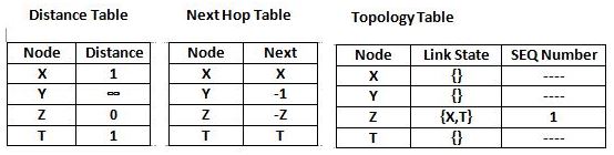
GSR protocol uses and maintains three tables for every node individually. These tables are:

Distance Table : This table contains the distance of a node from all the nodes in network.

Global State Routing : Distance Table
Topology Table : This table contains the information of Link state data along with the sequence number which can be used to determine when the information is updated last.

Global State Routing : Topology Table
Next Hop Table : Next hop table will contain the information about the immediate neighbor of a particular node.

Global State Routing : Next Hop Table

These tables are updated on every step and ensures that each node receives correct information about all the nodes including their distances.

GSR broadcasts the routing tables to its immediate neighbors rather than flooding it to all the nodes as Link State Routing protocol does.
Consider a network of 4 nodes having a distance of “1” on each of its edge. Below mentioned steps will let you know how GSR works and how its routing tables are updated.

Global State Routing : Example Network

For Node “X” : Firstly three tables as mentioned above will be maintained which includes distance table, Topology table and Next hop tables. This same process will be done for rest of the nodes too.

For X: Global State Routing : Sample Tables

Secondly, broadcasting of all the tables will be done to all the immediate neighbors of “X” i.e. “Y” and “Z”.
These tables are updated at “X”, “Y” & “T” nodes respectively.
Same will be done for node “Y”. After first updation from “X”, node “Y” will broadcast the tables to its immediate neighbors i.e. “X” & “T” and those tables will be updated accordingly. This will be done for “T” & “Z” also.
Once done, all the nodes “X”, “Y”, “Z” & “T” will be having the updated routing tables containing distances from each, with the help of which an optimal path can be chosen if data needs to be transferred from one node to other.